Step 1: Prepare the input dataset for ML modeling#
The project is based on the Heart Failure Prediction Dataset.
This first notebook:
Performs a quick exploratory analysis of the input dataset: it looks at the structure of the dataset and the distribution of the values in the different categorical and continuous columns.
Uses the functions from the project Python library to clean & prepare the input dataset before Machine Learning modeling. We will first clean categorical and continuous columns, then split the dataset into a train set and a test set.
Finally, we will transform this notebook into a Python recipe in the project Flow that will output the new train and test datasets.
Tip: The project libraries allow you to build shared code repositories. They can be synchronized with an external Git repository.
0. Import packages#
Make sure you’re using the ``heart-attack-project`` code environment (see prerequisites)
%pylab inline
Populating the interactive namespace from numpy and matplotlib
import dataiku
from dataiku import pandasutils as pdu
import pandas as pd
import matplotlib.pyplot as plt
import seaborn as sns
import math
from heart_attack_library import data_processing
from sklearn.preprocessing import RobustScaler
from sklearn.model_selection import train_test_split
/Users/clemencebic/dataiku/dss_instances/data_dir_dss11/code-envs/python/heart-attack-project/lib/python3.7/site-packages/pandas/compat/__init__.py:117: UserWarning: Could not import the lzma module. Your installed Python is incomplete. Attempting to use lzma compression will result in a RuntimeError.
  warnings.warn(msg)
/Users/clemencebic/dataiku/dss_instances/data_dir_dss11/code-envs/python/heart-attack-project/lib/python3.7/site-packages/seaborn/rcmod.py:82: DeprecationWarning: distutils Version classes are deprecated. Use packaging.version instead.
  if LooseVersion(mpl.__version__) >= "3.0":
/Users/clemencebic/dataiku/dss_instances/data_dir_dss11/code-envs/python/heart-attack-project/lib/python3.7/site-packages/setuptools/_distutils/version.py:346: DeprecationWarning: distutils Version classes are deprecated. Use packaging.version instead.
  other = LooseVersion(other)
import warnings
warnings.filterwarnings('ignore')
1. Import the data#
Let’s use the Dataiku Python API to import the input dataset. This piece of code allows retrieving data in the same manner, no matter where the dataset is stored (local filesystem, SQL database, Cloud data lakes, etc.)
dataset_heart_measures = dataiku.Dataset("heart_measures")
df = dataset_heart_measures.get_dataframe(limit=100000)
2. A quick audit of the dataset#
2.1 Compute the shape of the dataset#
print(f'The shape of the dataset is {df.shape}')
The shape of the dataset is (918, 12)
2.2 Look at a preview of the first rows of the dataset#
df.head()
| Age | Sex | ChestPainType | RestingBP | Cholesterol | FastingBS | RestingECG | MaxHR | ExerciseAngina | Oldpeak | ST_Slope | HeartDisease | |
|---|---|---|---|---|---|---|---|---|---|---|---|---|
| 0 | 40 | M | ATA | 140 | 289 | 0 | Normal | 172 | N | 0.0 | Up | 0 |
| 1 | 49 | F | NAP | 160 | 180 | 0 | Normal | 156 | N | 1.0 | Flat | 1 |
| 2 | 37 | M | ATA | 130 | 283 | 0 | ST | 98 | N | 0.0 | Up | 0 |
| 3 | 48 | F | ASY | 138 | 214 | 0 | Normal | 108 | Y | 1.5 | Flat | 1 |
| 4 | 54 | M | NAP | 150 | 195 | 0 | Normal | 122 | N | 0.0 | Up | 0 |
2.3 Inspect missing values & number of distinct values (cardinality) for each column#
pdu.audit(df)
| _a_variable | _b_data_type | _c_cardinality | _d_missings | _e_sample_values | |
|---|---|---|---|---|---|
| 0 | Age | int64 | 50 | 0 | [40, 49] |
| 1 | Sex | object | 2 | 0 | [M, F] |
| 2 | ChestPainType | object | 4 | 0 | [ATA, NAP] |
| 3 | RestingBP | int64 | 67 | 0 | [140, 160] |
| 4 | Cholesterol | int64 | 222 | 0 | [289, 180] |
| 5 | FastingBS | int64 | 2 | 0 | [0, 1] |
| 6 | RestingECG | object | 3 | 0 | [Normal, ST] |
| 7 | MaxHR | int64 | 119 | 0 | [172, 156] |
| 8 | ExerciseAngina | object | 2 | 0 | [N, Y] |
| 9 | Oldpeak | float64 | 53 | 0 | [0.0, 1.0] |
| 10 | ST_Slope | object | 3 | 0 | [Up, Flat] |
| 11 | HeartDisease | int64 | 2 | 0 | [0, 1] |
3. Exploratory data analysis#
3.1 Define categorical & continuous columns#
categorical_cols = ['Sex','ChestPainType', 'FastingBS', 'RestingECG', 'ExerciseAngina', 'ST_Slope']
continuous_cols = ['Age', 'RestingBP', 'Cholesterol', 'MaxHR', 'Oldpeak']
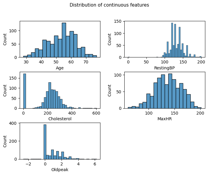
3.2 Look at the distibution of continuous features#
nb_cols=2
fig = plt.figure(figsize=(8,6))
fig.suptitle('Distribution of continuous features', fontsize=11)
gs = fig.add_gridspec(math.ceil(len(continuous_cols)/nb_cols),nb_cols)
gs.update(wspace=0.3, hspace=0.4)
for i, col in enumerate(continuous_cols):
    ax = fig.add_subplot(gs[math.floor(i/nb_cols),i%nb_cols])
    sns.histplot(df[col], ax=ax)
3.3 Look at the distribution of categorical columns#
nb_cols=2
fig = plt.figure(figsize=(8,6))
fig.suptitle('Distribution of categorical features', fontsize=11)
gs = fig.add_gridspec(math.ceil(len(categorical_cols)/nb_cols),nb_cols)
gs.update(wspace=0.3, hspace=0.4)
for i, col in enumerate(categorical_cols):
    ax = fig.add_subplot(gs[math.floor(i/nb_cols),i%nb_cols])
    plot = sns.countplot(df[col])
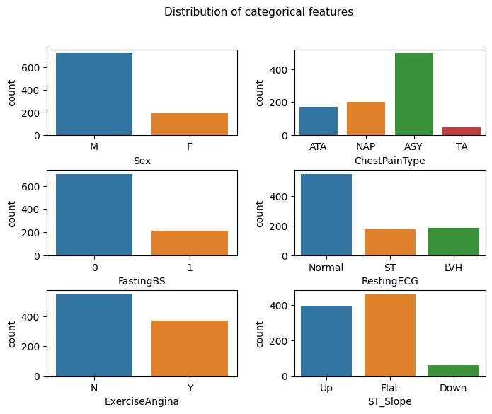
3.4 Look at the distribution of target variable#
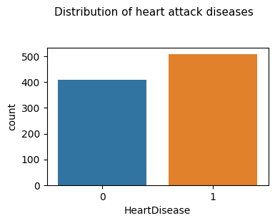
target = "HeartDisease"
fig = plt.figure(figsize=(4,2.5))
fig.suptitle('Distribution of heart attack diseases', fontsize=11, y=1.11)
plot = sns.countplot(df[target])
Tip: To ease collaboration, all the insights you create from Jupyter Notebooks can be shared with other users by publishing them on dashboards. See documentation for more information.
4. Prepare data#
4.1 Clean categorical columns#
# Transform string values from categorical columns into int, using the functions from the project libraries
df_cleaned = data_processing.transform_heart_categorical_measures(df, "ChestPainType", "RestingECG",
                                                                  "ExerciseAngina", "ST_Slope", "Sex")

df_cleaned.head()
| Age | Sex | ChestPainType | RestingBP | Cholesterol | FastingBS | RestingECG | MaxHR | ExerciseAngina | Oldpeak | ST_Slope | HeartDisease | |
|---|---|---|---|---|---|---|---|---|---|---|---|---|
| 0 | 40 | 0 | 2 | 140 | 289 | 0 | 0 | 172 | 0 | 0.0 | 2 | 0 |
| 1 | 49 | 1 | 3 | 160 | 180 | 0 | 0 | 156 | 0 | 1.0 | 1 | 1 |
| 2 | 37 | 0 | 2 | 130 | 283 | 0 | 1 | 98 | 0 | 0.0 | 2 | 0 |
| 3 | 48 | 1 | 4 | 138 | 214 | 0 | 0 | 108 | 1 | 1.5 | 1 | 1 |
| 4 | 54 | 0 | 3 | 150 | 195 | 0 | 0 | 122 | 0 | 0.0 | 2 | 0 |
4.2 Transform categorical columns into dummies#
df_cleaned = pd.get_dummies(df_cleaned, columns = categorical_cols, drop_first = True)

print("Shape after dummies transformation: " + str(df_cleaned.shape))
Shape after dummies transformation: (918, 16)
4.3 Scale continuous columns#
Let’s use the Scikit-Learn Robust Scaler to scale continuous features
scaler = RobustScaler()
df_cleaned[continuous_cols] = scaler.fit_transform(df_cleaned[continuous_cols])
5. Split the dataset into train and test#
Let’s now split the dataset into a train set that will be used for experimenting and training the Machine Learning models and test set that will be used to evaluate the deployed model.
heart_measures_train_df, heart_measures_test_df = train_test_split(df_cleaned, test_size=0.2, stratify=df_cleaned.HeartDisease)
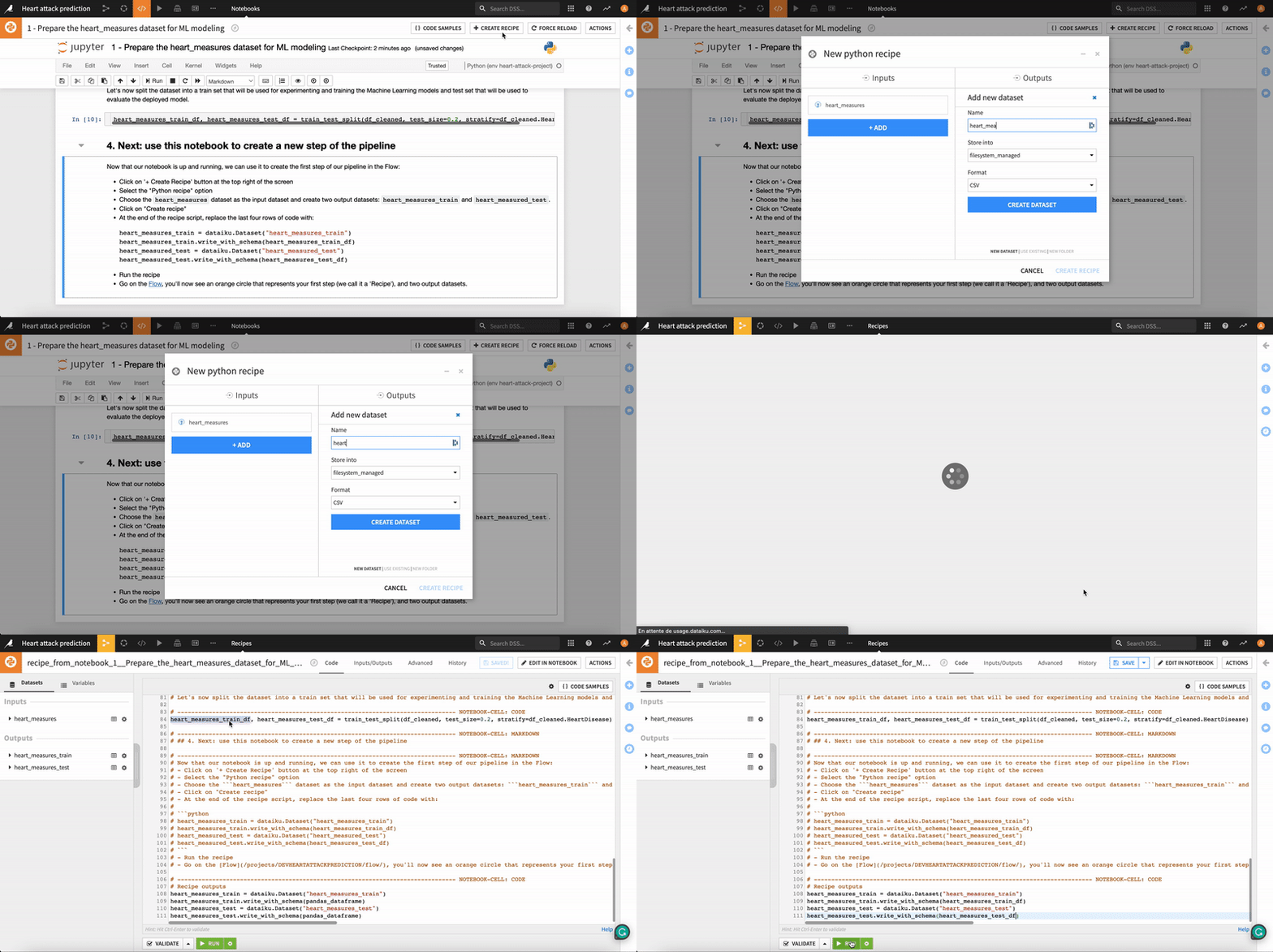
6. Next: use this notebook to create a new step in the project workflow#
Now that our notebook is up and running, we can use it to create the first step of our pipeline in the Flow:
Click on the + Create Recipe button at the top right of the screen.
Select the Python recipe option.
Choose the
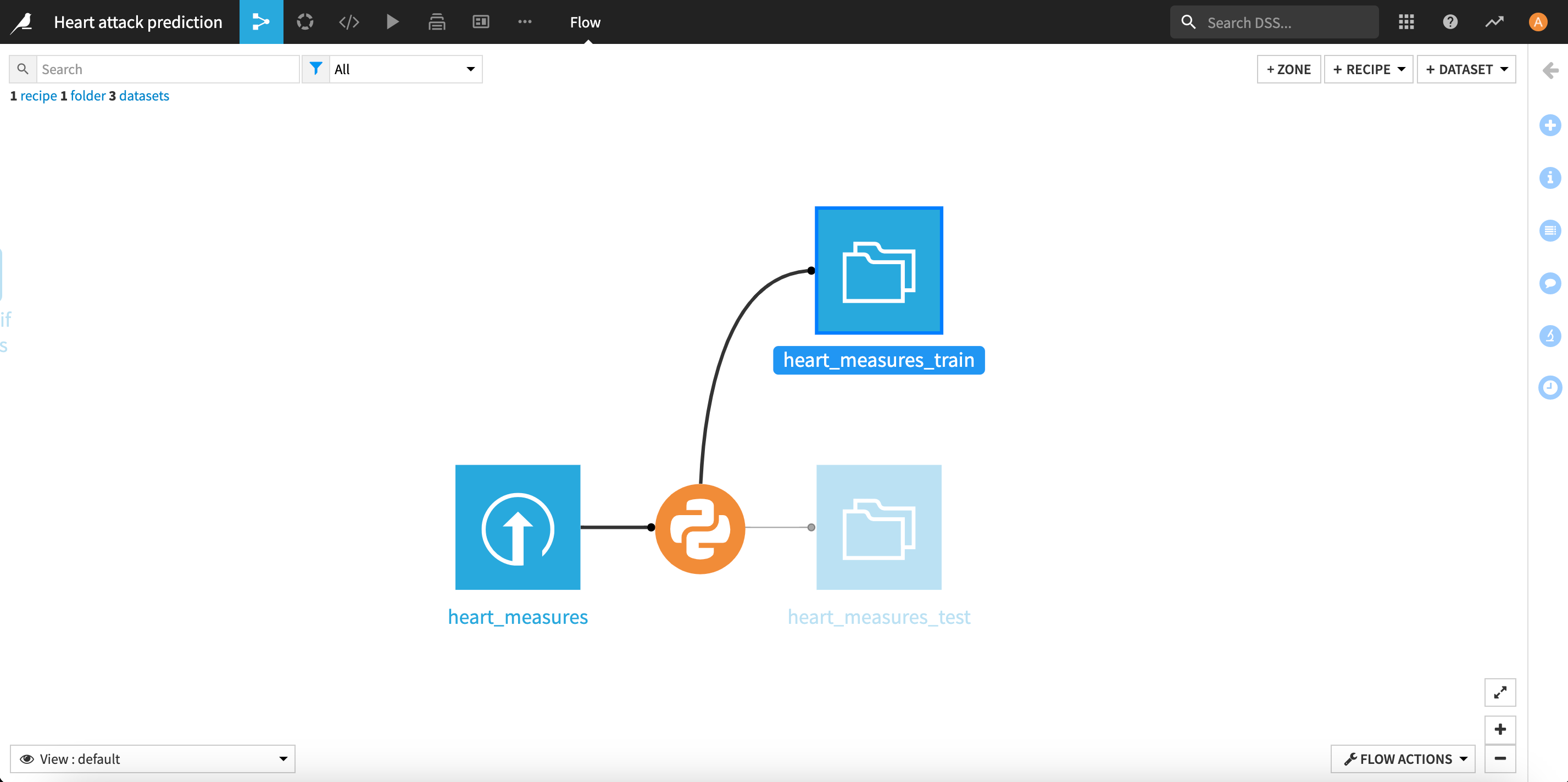
heart_measuresdataset as the input dataset and create two output datasets:heart_measures_trainandheart_measures_test.Click on the Create recipe button.
At the end of the recipe script, replace the last four rows of code with:
heart_measures_train = dataiku.Dataset("heart_measures_train")
heart_measures_train.write_with_schema(heart_measures_train_df)
heart_measured_test = dataiku.Dataset("heart_measures_test")
heart_measured_test.write_with_schema(heart_measures_test_df)
Run the recipe
Success: We can now go on the Flow, we’ll see an orange circle that represents your first step (we call it a ‘Recipe’), and two output datasets.
The Flow should now look like that:
