

Pre-training Large Language Models in Dataiku#
Large Language Models (LLMs) are at the heart of AI systems, but we often aren’t exposed to how these powerful models are created. LLMs require vast amounts of data and computational resources to learn how to perform tasks like text generation. This process generally involves several stages:
Pre-training: training a model, typically a neural network, on massive amounts of data to learn language patterns, semantics, and world knowledge. This phase creates a model that can predict the next token, but we need to refine how it generates tokens to better suit its role.
Fine-tuning and Alignment: taking a pre-trained model and aligning it to its desired use case by training it on specialized data using techniques like supervised fine-tuning (SFT) and reinforcement learning from human feedback (RLHF). These techniques transition a general next-token predictor into a helpful assistant.
In this tutorial, we will show how to pre-train models in Dataiku. We will reference Andrej Karpathy’s GitHub repository nanoGPT, which demonstrates how to pre-train an LLM.
By following the GitHub repository, you can reproduce OpenAI’s GPT-2 (124M parameters) if you use OpenWebText data, the same hyperparameters, and train the model on 8 NVIDIA A100 GPUs for about four days. For our purpose of pre-training an LLM in Dataiku, we will adjust scripts to run smoothly, use a smaller training dataset, and modify the hyperparameters so that training can be completed more quickly on a single, smaller GPU.
Prerequisites#
Dataiku >= 14.1
Python >= 3.12
- A code environment with:
Container runtime additions: “GPU support for Torch 2” (in Containerized execution)
The following packages:
tiktoken                    # tested with 0.11.0
torch                       # tested with 2.9.0
transformers[torch]         # tested with 4.57.1
ragas                       # tested with 0.2.12
langchain                   # tested with 0.3.27
numpy<1.27                  #  tested with 1.26.4
bert-score
sacrebleu
rouge-score
scikit-learn>=1.1,<1.7      # tested with 1.6.1
Access to a GPU (without a GPU, you likely won’t be able to train the required models, even with small hyperparameters)
Important
In this tutorial, we use a local filesystem to store the managed folders. If you change to cloud storage like S3, the way you read/write files will be slightly different.
Importing Code from GitHub to Project Library#
Before we start building our Flow, we will need to import code from GitHub into the project libraries section of our project. As mentioned earlier, we will use several scripts from Andrej Karpathy’s GitHub repository nanoGPT to pre-train our own model. To do this in Dataiku, we can create a Git reference that links to the nanoGPT repository and allows us to import components from the nanoGPT repository.
To import the code:
Click on the Code menu (</>)
Go to Libraries
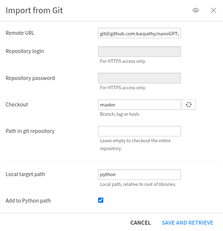
Click on Git, and select Import from Git…
- Use the following to fill in the blank fields
Remote URL:
git@github.com:karpathy/nanoGPT.gitCheckout:
masterLocal target path:
python
Now, you should have the entire nanoGPT repository stored under your python folder in your project library.
For this tutorial, we will use the model.py file.
This script defines a neural network with a transformer deep learning architecture
that we will train to create a Generative Pre-trained Transformer (GPT) language model.
The transformer architecture enables the model to generate coherent text
by capturing long-range dependencies between words,
which builds the model’s conceptual understanding of relationships between concepts, language, and world knowledge.
Importing the training data#
The pre-training phase typically requires training our model on data collected from the entire internet. To get results similar to OpenAI’s GPT-2 (124M parameters), you would need to train on OpenWebText data, which is 41.70 GB. To avoid running into computational bottlenecks, we will instead use a file containing all of Shakespeare’s work as our pre-training dataset.
Let’s retrieve this dataset using Dataiku’s “Download” recipe:
Add a Download recipe to your Flow.
Set the output folder name to
docs_raw_shakespeare.Save into the server’s filesystem.
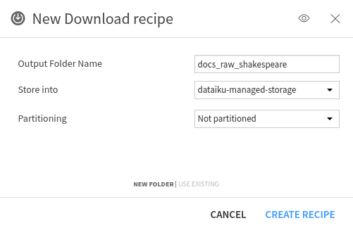
Click the Create recipe button.
Then click the + Add a first source button.
- And fill the form with:
URL:
https://raw.githubusercontent.com/karpathy/char-rnn/master/data/tinyshakespeare/input.txt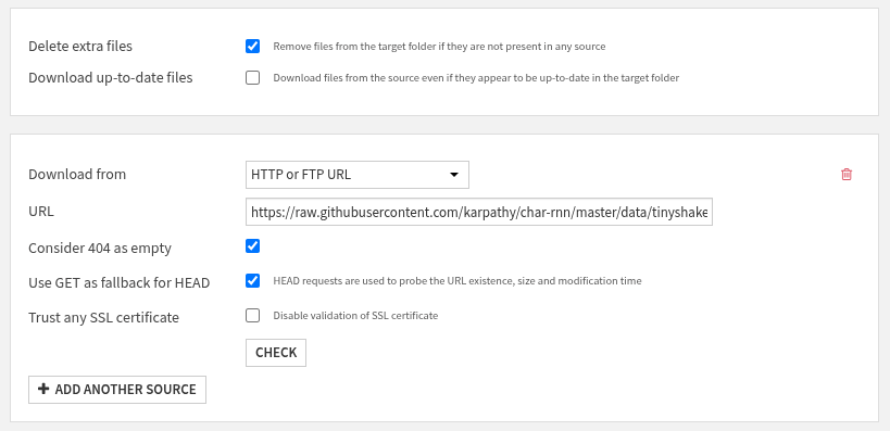
Now, you should have a file called input.txt that is 1.06 MB in size, saved in your docs_raw_shakespeare folder.
Preparing the Data#
Collecting ample amounts of data for pre-training is only part of the work.
You will need to prepare it and transform it into a suitable format for model training.
To do this, we will create a Python Code Recipe with docs_raw_shakespeare as the Input
and docs_prepared_shakespeare, a new Managed Folder that will reside in the server’s filesystem, as the Output.
The aim of the Python recipe is to split our Shakespeare data into a training set and a validation set,
encode text into subword tokens, and save the datasets in our new output Managed Folder.
import os
import dataiku
import requests
import tiktoken
import numpy as np

# 1. Read in the tiny shakespeare dataset
docs_raw_shakespeare = dataiku.Folder("docs_raw_shakespeare")
folder_path = docs_raw_shakespeare.get_path()  # local filesystem path
file_path = os.path.join(folder_path, "input.txt")

with open(file_path, 'r', encoding='utf-8') as f:
    data = f.read()

# 2. Split data into 90% training data and 10% validation data
n = len(data)
train_data = data[:int(n*0.9)]
val_data = data[int(n*0.9):]

# 3. Encode with tiktoken gpt2 bpe
enc = tiktoken.get_encoding("gpt2")
train_ids = enc.encode_ordinary(train_data)
val_ids = enc.encode_ordinary(val_data)

# 4. Export to bin files
train_ids = np.array(train_ids, dtype=np.uint16)
val_ids = np.array(val_ids, dtype=np.uint16)

# 5. Save bin files to Managed Folder
docs_prepared_shakespeare = dataiku.Folder("docs_prepared_shakespeare")
with docs_prepared_shakespeare.get_writer("train.bin") as w:
    w.write(train_ids)
with docs_prepared_shakespeare.get_writer("val.bin") as w:
    w.write(val_ids)
Training the Language Model#
We have defined our transformer-based neural network in model.py
and prepared a training and validation set.
Now, it’s time for us to train our neural network on Shakespeare
and create an LLM capable of generating Shakespeare-like text.
We will create a training script using a Python code recipe.
The Input will be docs_prepared_shakespeare,
and the Output will be models_shakespeare, a new Managed Folder in the server’s filesystem.
We will use the train.py script from the nanoGPT repository with some adjustments.
The primary adjustments will be saving our artifacts in Managed Folders rather than on the local machine
and adjusting the hyperparameters to train a smaller GPT model.
Let’s take a look at the components that make up the training script.
Note
For this code recipe, we will use our GPU container to train our model on a GPU.
The first section of the code imports the necessary libraries.
We are also importing GPTConfig and GPT from the model.py file in the project library.
GPT is the model class that defines the neural network that implements the GPT architecture.
The GPTConfig is a configuration class that contains hyperparameters for the GPT model.
import os
import time
import math
import pickle
from contextlib import nullcontext
import tempfile
import shutil

import dataiku
import numpy as np
import torch
from torch.distributed import init_process_group, destroy_process_group

from model import GPT, GPTConfig
Next, we define our input and output Managed Folder. The input folder is where the training and validation data are stored. The output folder is where we will store our PyTorch checkpoint file, which contains a dictionary with information such as model weights and training metadata. Later, we can load these model weights and use them for inference to generate text or fine-tune the model for a specific task.
# Connect to the input and output Managed Folders
docs_prepared_shakespeare = dataiku.Folder("docs_prepared_shakespeare")
models_shakespeare = dataiku.Folder("models_shakespeare")

# Define model hyperparameters to train a mini Shakespeare model
eval_interval = 250 # keep frequent because we'll overfit
eval_iters = 200
eval_only = False # if True, script exits right after the first eval
log_interval = 10 # don't print too too often

# we expect to overfit on this small dataset, so only save when val improves
always_save_checkpoint = False
init_from = 'scratch' # 'scratch' or 'resume' or 'gpt2*'

gradient_accumulation_steps = 1
batch_size = 12
block_size = 64 # context of up to 256 previous characters

# baby GPT model :)
n_layer = 4
n_head = 4
n_embd = 128
dropout = 0.2
bias = False # do we use bias inside LayerNorm and Linear layers?

learning_rate = 1e-3 # with baby networks can afford to go a bit higher
max_iters = 2000
weight_decay = 1e-1
min_lr = 1e-4 # learning_rate / 10 usually
beta1 = 0.9
beta2 = 0.99 # make a bit bigger because the number of tokens per iter is small
grad_clip = 1.0 # clip gradients at this value, or disable if == 0.0

# learning rate decay settings
decay_lr = True # whether to decay the learning rate
warmup_iters = 100 # not super necessary, potentially
lr_decay_iters = 2000 # make equal to max_iters usually
min_lr = 6e-5 # minimum learning rate, should be ~= learning_rate/10 per Chinchilla
device = "cuda"
dtype = 'bfloat16' if torch.cuda.is_available() and torch.cuda.is_bf16_supported() else 'float16' # 'float32', 'bfloat16', or 'float16', the latter will auto implement a GradScaler
compile = True

# This will store all hyperparameters, which will be useful for logging
config_keys = [k for k,v in globals().items() if not k.startswith('_') and isinstance(v, (int, float, bool, str))]
config = {k: globals()[k] for k in config_keys}
Here, we are calculating the total number of tokens processed in one optimization step. We also ensure reproducible results by assigning a fixed random seed and identifying the computational device available to us (CPU or GPU with CUDA).
tokens_per_iter = gradient_accumulation_steps * batch_size * block_size
print(f"tokens per iteration will be: {tokens_per_iter:,}")
torch.manual_seed(1337)
torch.backends.cuda.matmul.allow_tf32 = True # allow tf32 on matmul
torch.backends.cudnn.allow_tf32 = True # allow tf32 on cudnn
device_type = 'cuda' if 'cuda' in device else 'cpu' # for later use in torch.autocast
# note: float16 data type will automatically use a GradScaler
ptdtype = {'float32': torch.float32, 'bfloat16': torch.bfloat16, 'float16': torch.float16}[dtype]
ctx = nullcontext() if device_type == 'cpu' else torch.amp.autocast(device_type=device_type, dtype=ptdtype)
Now, we define two helper functions:
get_memmap_from_folder: this function downloads a binary file from a Managed Folder, writes it locally, and returns anp.memmapview of the file for efficient reading of the dataset.get_batch: This function is a simple data loader that usesnp.memmapto loadtrain.binandval.bin, generating a batch of input sequences x and next-token targets y.
def get_memmap_from_folder(folder, filename, dtype, mode='r'):
    """Download stream → write to temp file → memory‑map"""
    with folder.get_download_stream(filename) as stream:
        # create a temp file
        tmp_path = os.path.join(tempfile.mkdtemp(), filename)
        with open(tmp_path, "wb") as f:
            f.write(stream.read())
    # memory‑map the temp file
    return np.memmap(tmp_path, dtype=dtype, mode=mode)

def get_batch(split):
"""Generate a batch of inputs x and targets y"""
# We recreate np.memmap every batch to avoid a memory leak, as per
# https://stackoverflow.com/questions/45132940/numpy-memmap-memory-usage-want-to-iterate-once/61472122#61472122
if split == 'train':
    data = get_memmap_from_folder(docs_prepared_shakespeare, "train.bin", dtype=np.uint16, mode='r')
else:
    data = get_memmap_from_folder(docs_prepared_shakespeare, "val.bin", dtype=np.uint16, mode='r')

ix = torch.randint(len(data) - block_size, (batch_size,))
x = torch.stack([torch.from_numpy((data[i:i+block_size]).astype(np.int64)) for i in ix])
y = torch.stack([torch.from_numpy((data[i+1:i+1+block_size]).astype(np.int64)) for i in ix])
if device_type == 'cuda':
    # pin arrays x,y, which allows us to move them to GPU asynchronously (non_blocking=True)
    x, y = x.pin_memory().to(device, non_blocking=True), y.pin_memory().to(device, non_blocking=True)
else:
    x, y = x.to(device), y.to(device)
return x, y
Next, we will set up the model’s initial state and training components.
We are initializing counters and metrics, such as iter_num and best_val_loss.
We are also setting model configurations and instantiating a new GPT model from scratch,
using the architecture parameters we set earlier.
# init these up here
iter_num = 0
best_val_loss = 1e9
meta_vocab_size = None

# model init
model_args = dict(n_layer=n_layer, n_head=n_head, n_embd=n_embd, block_size=block_size,
                  bias=bias, vocab_size=None, dropout=dropout) # start with model_args from command line

# init a new model from scratch
print("Initializing a new model from scratch")
# determine the vocab size we'll use for from-scratch training
if meta_vocab_size is None:
    print("defaulting to vocab_size of GPT-2 to 50304 (50257 rounded up for efficiency)")
model_args['vocab_size'] = meta_vocab_size if meta_vocab_size is not None else 50304
gptconf = GPTConfig(**model_args)
model = GPT(gptconf)

# crop down the model block size if desired, using model surgery
if block_size < model.config.block_size:
    model.crop_block_size(block_size)
    model_args['block_size'] = block_size # so that the checkpoint will have the right value
model.to(device)

# initialize a GradScaler. If enabled=False scaler is a no-op
scaler = torch.cuda.amp.GradScaler(enabled=(dtype == 'float16'))

# optimizer
optimizer = model.configure_optimizers(weight_decay, learning_rate, (beta1, beta2), device_type)
if init_from == 'resume':
    optimizer.load_state_dict(checkpoint['optimizer'])
checkpoint = None # free up memory
# compile the model
if compile:
    print("compiling the model... (takes a ~minute)")
    unoptimized_model = model
    model = torch.compile(model) # requires PyTorch 2.0
Before we train the newly instantiated GPT model, we will define two more helper functions:
estimate_loss: This function calculates the average loss for both train and validation splits over multiple mini-batches.get_lr: This function implements a learning rate decay scheduler that, after a linear warmup, decays the learning rate with cosine decay to a minimum learning rate.
# helps estimate an arbitrarily accurate loss over either split using many batches
@torch.no_grad()
def estimate_loss():
    out = {}
    model.eval()
    for split in ['train', 'val']:
        losses = torch.zeros(eval_iters)
        for k in range(eval_iters):
            X, Y = get_batch(split)
            with ctx:
                logits, loss = model(X, Y)
            losses[k] = loss.item()
        out[split] = losses.mean()
    model.train()
    return out

# learning rate decay scheduler (cosine with warmup)
def get_lr(it):
    # 1) linear warmup for warmup_iters steps
    if it < warmup_iters:
        return learning_rate * (it + 1) / (warmup_iters + 1)
    # 2) if it > lr_decay_iters, return min learning rate
    if it > lr_decay_iters:
        return min_lr
    # 3) in between, use cosine decay down to min learning rate
    decay_ratio = (it - warmup_iters) / (lr_decay_iters - warmup_iters)
    assert 0 <= decay_ratio <= 1
    coeff = 0.5 * (1.0 + math.cos(math.pi * decay_ratio)) # coeff ranges 0..1
    return min_lr + coeff * (learning_rate - min_lr)
Now, we can train our GPT language model. During training, we adjust the model weights to minimize the cross-entropy loss. At a high level, here are the steps in the training loop:
Fetch a batch of training data.
Determine and update the learning rate.
Periodic computations of average train/validation cross-entropy loss and save to checkpoint.
Compute forward pass (model computes prediction and loss) and backward pass (use backpropagation to compute gradients of the loss with respect to each model parameter).
Use gradient clipping to prevent large updates to the model’s parameters.
Log current loss, counters, iteration time, and Model FLOPs Utilization (MFU).
Increase the iteration counter until we reach the maximum number of training iterations.
# training loop
X, Y = get_batch('train') # fetch the very first batch
t0 = time.time()
local_iter_num = 0 # number of iterations in the lifetime of this process
raw_model = model
running_mfu = -1.0
while True:

    # determine and set the learning rate for this iteration
    lr = get_lr(iter_num) if decay_lr else learning_rate
    for param_group in optimizer.param_groups:
        param_group['lr'] = lr

    # evaluate the loss on train/val sets and write checkpoints
    if iter_num % eval_interval == 0:
        losses = estimate_loss()
        print(f"step {iter_num}: train loss {losses['train']:.4f}, val loss {losses['val']:.4f}")
        if losses['val'] < best_val_loss or always_save_checkpoint:
            best_val_loss = losses['val']
            if iter_num > 0:
                checkpoint = {
                    'model': raw_model.state_dict(),
                    'optimizer': optimizer.state_dict(),
                    'model_args': model_args,
                    'iter_num': iter_num,
                    'best_val_loss': best_val_loss,
                    'config': config,
                }
                print(f"saving to local checkpoint")
                # write to local temp file
                tmp_ckpt = os.path.join(tempfile.mkdtemp(), "ckpt.pt")
                torch.save(checkpoint, tmp_ckpt)
                # upload to managed folder
                with models_shakespeare.get_writer("ckpt.pt") as f:
                    with open(tmp_ckpt, "rb") as lf:
                        shutil.copyfileobj(lf, f)
    if iter_num == 0 and eval_only:
        break

    # forward backward update, with optional gradient accumulation to simulate larger batch size
    # and using the GradScaler if data type is float16
    for micro_step in range(gradient_accumulation_steps):
        with ctx:
            logits, loss = model(X, Y)
            loss = loss / gradient_accumulation_steps # scale the loss to account for gradient accumulation
        # immediately async prefetch next batch while model is doing the forward pass on the GPU
        X, Y = get_batch('train')
        # backward pass, with gradient scaling if training in fp16
        scaler.scale(loss).backward()
    # clip the gradient
    if grad_clip != 0.0:
        scaler.unscale_(optimizer)
        torch.nn.utils.clip_grad_norm_(model.parameters(), grad_clip)
    # step the optimizer and scaler if training in fp16
    scaler.step(optimizer)
    scaler.update()
    # flush the gradients as soon as we can, no need for this memory anymore
    optimizer.zero_grad(set_to_none=True)

    # timing and logging
    t1 = time.time()
    dt = t1 - t0
    t0 = t1
    if iter_num % log_interval == 0:
        # get loss as float. note: this is a CPU-GPU sync point
        # scale up to undo the division above, approximating the true total loss (exact would have been a sum)
        lossf = loss.item() * gradient_accumulation_steps
        if local_iter_num >= 5: # let the training loop settle a bit
            mfu = raw_model.estimate_mfu(batch_size * gradient_accumulation_steps, dt)
            running_mfu = mfu if running_mfu == -1.0 else 0.9*running_mfu + 0.1*mfu
        print(f"iter {iter_num}: loss {lossf:.4f}, time {dt*1000:.2f}ms, mfu {running_mfu*100:.2f}%")
    iter_num += 1
    local_iter_num += 1

    # termination conditions
    if iter_num > max_iters:
        break
Job Monitoring#
After we initiate the training of our model, we can take a closer look at what is going on behind the scenes. Dataiku automatically tracks detailed activity logs for every single job that runs on the platform. We can review the logs for our training job to retrieve detailed information about how our job is progressing. To do that, we will need to navigate to the Jobs tab by:
Hitting the play button in the black navigation bar
Selecting Jobs
Clicking on your training job
Clicking VIEW LOGS
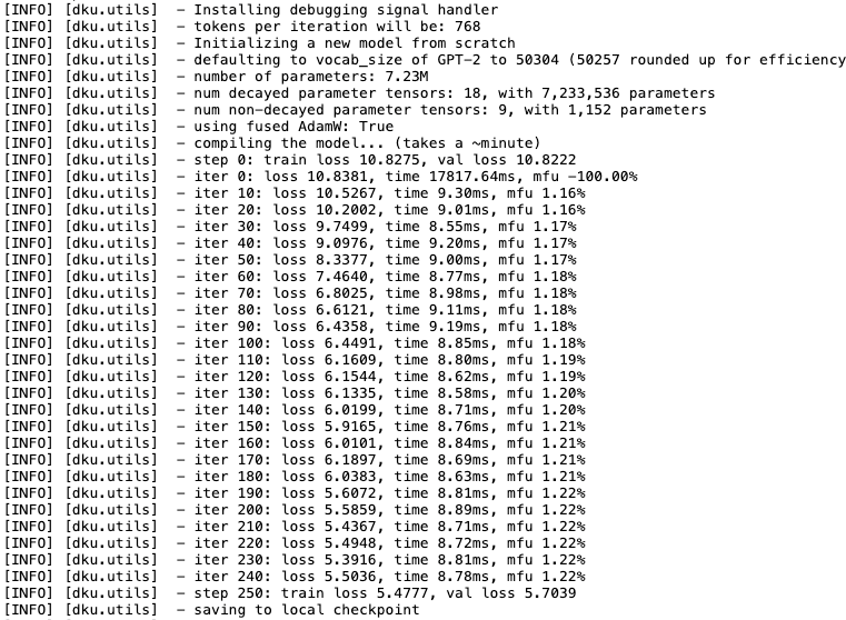
Clicking the arrow next to Activity Log
We are capturing key metrics at a regular interval. As the model continues to update its weights, the cross-entropy loss continues to decrease. We are tracking iteration time for each training loop and Model FLOPs Utilization (MFU), which measures the efficiency of model training. We also see when the model saves a checkpoint.
Text Generation with the Pre-trained LLM#
Now that we have our pre-trained model, we can use it to generate new text.
We essentially have a Shakespeare writer LLM capable of generating Shakespeare-like text.
We will provide our pre-trained LLM with various types of prompts and observe its behavior.
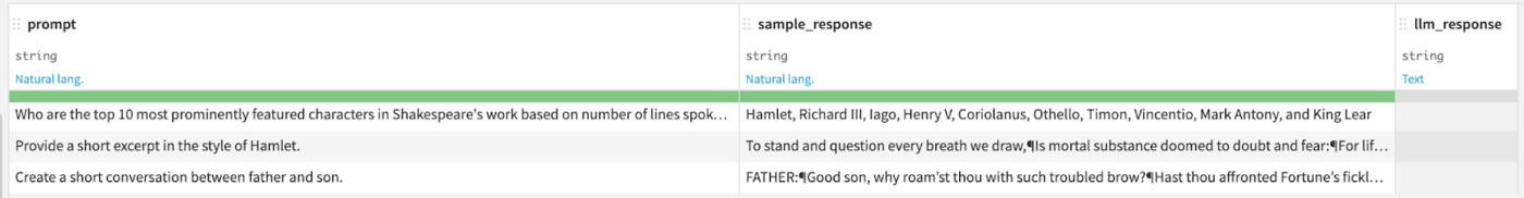
To do that, let’s first create a new Editable dataset called example_prompts_shakespeare
with three columns: prompts, sample_response, and llm_response.
Below, we have three example prompts and sample response pairs that you can add as new rows to your editable dataset.
Example 1#
Prompt: Who are the top 10 most prominently featured characters in Shakespeare’s work based on number of lines spoken?
Sample Response:
Example 2#
Prompt: Provide a short excerpt in the style of Hamlet.
Sample Response:
Example 3#
Prompt: Create a short conversation between father and son.
Sample Response:
Next, we will create a Python code recipe that uses our pre-trained LLM
and the given prompts to populate the llm_response column.
Select the Managed Folder models_shakespeare
and the Editable dataset example_prompts_shakespeare,
then create a Python Code recipe,
set the Output to a new Dataset called llm_responses_shakespeare (in CSV format),
saved into the server’s filesystem.
The first step in our Python code recipe is to import the necessary packages and read the recipe inputs.
import dataiku
import os
import pickle
from contextlib import nullcontext
import pandas as pd
import torch
import tiktoken
from model import GPTConfig, GPT

# Read recipe inputs
models_shakespeare = dataiku.Folder("models_shakespeare")

example_prompts_shakespeare = dataiku.Dataset("example_prompts_shakespeare")
example_prompts_shakespeare_df = example_prompts_shakespeare.get_dataframe()
The next step is to wrap our LLM inference logic in a for loop that iterates through our dataset,
using example prompts created earlier.
We are also setting key parameters like temperature and top-k that affect the output of our LLM
and setting PyTorch settings.
One other thing to note is that we are passing our example prompt as the start parameter.
for row in range(len(example_prompts_shakespeare_df)):

    # ------------------------------------------------------------------------
    init_from = 'resume' # either 'resume' (from an out_dir) or a gpt2 variant (e.g. 'gpt2-xl')
    out_dir = models_shakespeare.get_path() # ignored if init_from is not 'resume'
    start = example_prompts_shakespeare_df.loc[row, "prompt"] # or "<|endoftext|>" or etc. Can also specify a file, use as: "FILE:prompt.txt"
    num_samples = 1 # number of samples to draw
    max_new_tokens = 100 # number of tokens generated in each sample
    temperature = 0.7 # 1.0 = no change, < 1.0 = less random, > 1.0 = more random, in predictions
    top_k = 200 # retain only the top_k most likely tokens, clamp others to have 0 probability
    seed = 1337
    device = 'cpu' # examples: 'cpu', 'cuda', 'cuda:0', 'cuda:1', etc.
    dtype = 'bfloat16' if torch.cuda.is_available() and torch.cuda.is_bf16_supported() else 'float16' # 'float32' or 'bfloat16' or 'float16'
    compile = False # use PyTorch 2.0 to compile the model to be faster
    # -------------------------------------------------------------------------

    torch.manual_seed(seed)
    torch.cuda.manual_seed(seed)
    torch.backends.cuda.matmul.allow_tf32 = True # allow tf32 on matmul
    torch.backends.cudnn.allow_tf32 = True # allow tf32 on cudnn
    device_type = 'cuda' if 'cuda' in device else 'cpu' # for later use in torch.autocast
    ptdtype = {'float32': torch.float32, 'bfloat16': torch.bfloat16, 'float16': torch.float16}[dtype]
    ctx = nullcontext() if device_type == 'cpu' else torch.amp.autocast(device_type=device_type, dtype=ptdtype)
In the next section of the for loop, we initialize and compile our pre-trained LLM.
We saved our model under a file called ckpt.pt, so we will load that file.
We also need to load in the encodings we used during pre-training for inference.
We used GPT-2 encodings, and we will use them during inference to encode the prompt and decode the LLM response.
    # model
    if init_from == 'resume':
        # init from a model saved in a specific directory
        ckpt_path = os.path.join(out_dir, 'ckpt.pt')
        checkpoint = torch.load(ckpt_path, map_location=device)
        gptconf = GPTConfig(**checkpoint['model_args'])
        model = GPT(gptconf)
        state_dict = checkpoint['model']
        unwanted_prefix = '_orig_mod.'
        for k,v in list(state_dict.items()):
            if k.startswith(unwanted_prefix):
                state_dict[k[len(unwanted_prefix):]] = state_dict.pop(k)
        model.load_state_dict(state_dict)
    elif init_from.startswith('gpt2'):
        # init from a given GPT-2 model
        model = GPT.from_pretrained(init_from, dict(dropout=0.0))

    model.eval()
    model.to(device)
    if compile:
        model = torch.compile(model) # requires PyTorch 2.0 (optional)

    # look for the meta pickle in case it is available in the dataset folder
    load_meta = False
    if init_from == 'resume' and 'config' in checkpoint and 'dataset' in checkpoint['config']: # older checkpoints might not have these...
        meta_path = os.path.join('data', checkpoint['config']['dataset'], 'meta.pkl')
        load_meta = os.path.exists(meta_path)
    if load_meta:
        print(f"Loading meta from {meta_path}...")
        with open(meta_path, 'rb') as f:
            meta = pickle.load(f)
        # TODO want to make this more general to arbitrary encoder/decoder schemes
        stoi, itos = meta['stoi'], meta['itos']
        encode = lambda s: [stoi[c] for c in s]
        decode = lambda l: ''.join([itos[i] for i in l])
    else:
        # ok let's assume gpt-2 encodings by default
        print("No meta.pkl found, assuming GPT-2 encodings...")
        enc = tiktoken.get_encoding("gpt2")
        encode = lambda s: enc.encode(s, allowed_special={"<|endoftext|>"})
        decode = lambda l: enc.decode(l)

    # encode the beginning of the prompt
    if start.startswith('FILE:'):
        with open(start[5:], 'r', encoding='utf-8') as f:
            start = f.read()
    start_ids = encode(start)
    x = (torch.tensor(start_ids, dtype=torch.long, device=device)[None, ...])
The final section of the for loop generates new text, decodes it, and saves it to the llm_response column of our dataset alongside the prompts.
# run generation
with torch.no_grad():
    with ctx:
        y = model.generate(x, max_new_tokens, temperature=temperature, top_k=top_k)
        full_output = decode(y[0].tolist())

        if full_output.startswith(start):
            clean_output = full_output[len(start):].lstrip()
        else:
            clean_output = full_output
        example_prompts_shakespeare_df.loc[row, "llm_response"] = clean_output
After the code finishes iterating through the for loop,
we save the updated dataset into our output dataset llm_responses_shakespeare.
# Write recipe outputs
llm_responses_shakespeare = dataiku.Dataset("llm_responses_shakespeare")
llm_responses_shakespeare.write_with_schema(example_prompts_shakespeare_df)
Evaluating the LLM#
We successfully created new text using our pre-trained LLM.
That alone is a great achievement, but we will go one step further and evaluate our pre-trained LLM.
Our llm_responses_shakespeare has three columns: prompt, sample_response, and llm_response.
We can use those columns within an Evaluate LLM recipe to assess the performance of our pre-trained model.
It’s essential to note that we have a pre-trained model that can predict the next token; however, it is not yet configured to align with a specific use case and serve as a helpful assistant. This means our pre-trained model isn’t following the instructions provided in the prompt accurately. If we want our pre-trained model to be more useful to us, we need a post-training stage where we can fine-tune the model and align it to our requirements.
Let’s select the llm_responses_shakespeare dataset and add an Evaluate LLM recipe to our Flow.
This will automatically set llm_responses_shakespeare as an Input.
We will have three Outputs:
Output Dataset: This dataset will return our original columns plus new columns for each selected metric on a per-prompt/row basis. This allows us to understand the model’s performance on each individual example. Let’s call this
outputand save it as a CSV in the server’s filesystem.Metrics: This dataset returns one row per evaluation run, with aggregated (typically average) metrics across all prompts. This provides a summary of the model’s performance across the entire evaluation run. Let’s call this
metricsand save it as a CSV in the server’s filesystem.LLM Evaluation Store: This central repository stores all our LLM evaluation runs, including metrics, metadata, and visuals. This allows us to compare and track the performance of multiple evaluations over time. Let’s call this
llm_evaluation_store.
Let’s fill in the Evaluate LLM recipe as follows:
Input Dataset Format: Custom
Task: Other LLM Evaluation Task
Input column: prompt
Output column: llm_response
Ground truth column: sample_response
Sampling method: No sampling (whole data)
- Metrics to compute:
BERT Score
Answer correctness
Answer similarity
BLEU
ROUGE
Select an Embedding LLM and Completion LLM based on what is available to you
Select the appropriate code environment
Select a container with a GPU
After running the recipe, you should have three new objects in your Flow.
We can take a look at our pre-trained model’s performance by double-clicking the llm_evaluation_store object.
This provides us with an aggregated view of our LLM evaluation runs.
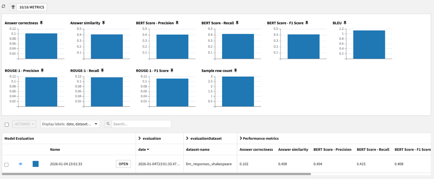
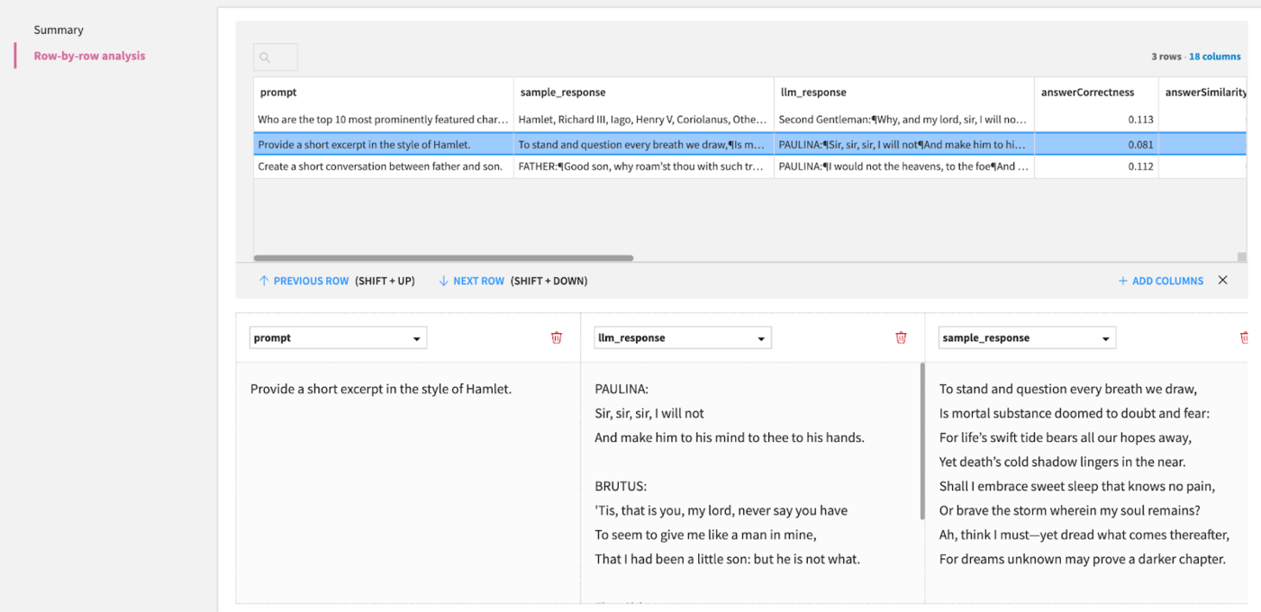
If we want a more granular view, we can click on the OPEN button, then click on Row-by-row analysis.
Conclusion#
In this tutorial, we successfully pre-trained a transformer-based neural network to create an LLM capable of generating coherent text. To get to this stage, we had to:
Define a neural network model with a transformer architecture.
Prepare a dataset by splitting into training and validation splits and encoding our text into tokens.
Train our model.
Monitor the model training job to ensure the model’s performance was gradually improving.
Evaluate the performance of our pre-trained LLM.
By completing the above steps, you gain full control over your training dataset, tokenizer, model architecture, and other design choices. This is particularly beneficial when working with proprietary data, addressing a niche use case that doesn’t require broad capabilities offered by standard foundation models, or mitigating the risk of system disruptions from future changes by third-party LLM providers.
As a next step, you could explore expanding what we’ve done here by:
Fine-tuning your pre-trained model to adapt it for a specific task using Dataiku’s Fine tune recipe.
Train on your own dataset or a popular dataset like OpenWebText.
Train a larger model across multiple GPUs.